

Bayesian Hyperparameter Optimization Using Optuna
Utilizing Full Potential of Computationally EXPENSIVE Neural Networks

As a data scientist, you never know the best value of your hyperparmeters to improve the performance of machine learning algorithms or statistical models.
Leveraging domain knowledge is crucial to create or defining a search space for your model to find the best parameter to either decrease the loss of the model or increase the performance metrics (eg. accuracy).
By the end of this read, you will have a solid understanding of:
What Optuna is?
Why it is essential for Hyperparameter Tuning? and,
How to implement it for Optimizing an ANN?
This is helpful for day-to-day work as a Data Scientist.
If you’re new here Subscribe, as my goal is to simplify Data Science for you. 👇🏻
Let’s dive in!
What is Optuna?
It is an open-source hyperparameter optimization framework that provides an efficient, flexible and easy-to-use tool for finding the best hyperparameters for your ML and DL models.
Why Use Optuna?
Traditional tools for hyperparameter tuning, namely, GridSearchCV and RandomSearchCV, are naive because they don’t explore the search space effectively and are highly inefficient as they require excessive computation power.
Optuna, on the the other hand, leverages Bayesian Optimization, Tree-structured Parzen Estimator (TPE), and other advanced techniques to efficiently navigate the hyperparameter space.
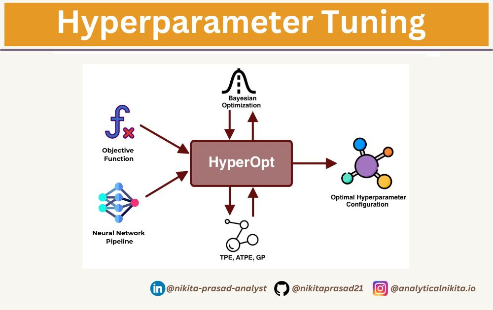
It is really helpful in reducing time as well as computational cost while achieving better results.
How to Use Optuna?
First, you need to install it using pip command:
!pip install optunaSecondly, you have to implement the below shown algorithm.
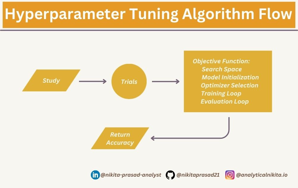
Let’s discuss the important key terms:
A study is an optimization session that is essentially a collection of trials aimed at optimizing the objective function.
The objective function defines the relationship between trial parameters (or simply called, hyperparameters), which need to be optimized (minimized or maximized) during the search process.


Lastly, you can either use MLflow or use optuna.visualization for understanding the output better through visuals.
My two favorites plots are:
1. Parallel Co-ordinate Plot
Using the code snippet below, you can plot the relation between objective value and all the trial pameters.
from optuna.visualization import plot_parallel_coordinate

plot_parallel_coordinate(study, params=["num_hidden_layers", "num_neurons_per", "epochs", "learning_rate", "dropout_rate", "batch_size", "optimizer", "weigh_decay"]).show()
According to this plot, the best values of the model are given by the dark blue lines, such as:
'num_hidden_layers' can be from 3 to 4,
'weigh_decay' is around 0.00090 - 0.00097
This is helpful in strategically planning the architecture of the model.
2. Plot Optimization History
This plot shows the relationship between the objective value (in this case, accuracy) and trial number.
from optuna.visualization import plot_optimization_history

plot_optimization_history(study).show()
As concluded from the plot, with an increase in the number of trials, accuracy improves. However, after 10th trial, it slightly decreases.
This is helpful in planning the number of trial to reduce compuational cost.
Note: Optuna's pruning mechanism improves efficiency by stopping poor trials early.
And that’s a wrap!
So, by integrating Optuna into your NN workflow, you can achieve higher accuracy with less effort and computational cost.
Also, if you’d like to explore the full implementation, including code and data, then checkout: Github Repository. 👈🏻
Next, I'll optimize this model using a CNN Architecture. Stay tuned with ME, so you won’t miss out on future updates.
Until next time, happy learning!