Open AI has finally introduced the much-awaited research preview of GPT‑4.5, claiming to be their most advanced model yet — with broader knowledge base, improved intent-following abilities, and greater “EQ” (Emotional Intelligence).
This motivates me to write a detailed yet crucial article on the fundamentals of Attention Mechanism— the core of GPT Models. Along with an implementation of a SimpleAttention Mechanism from scratch to truly understand how it works.
⏸️ Quick Pause: If you’re new here, I’d highly appreciate if you subscribe to recieve bi-weekly data tips and insights — directly into your inbox. 👇🏻
The Problem with Modeling Long Sequences
In tasks like machine translation, word-by-word translation doesn’t work because it requires contextual understanding and grammatical alignment between the source and target languages.
Prior to the introduction of transformer models, encoder-decoder RNNs were commonly used for machine translation tasks.
In this setup, the encoder processes a sequence of tokens from the source language, using a hidden state—a kind of intermediate layer within the neural network.
Leading to loss-of-context, especially in long complex sentences where dependencies might span long distances.
As the current hidden state is condensed representation of entire input sequence into single hidden state vector.
Solution? Self-Attention Mechanism!
What is the Self-Attention Mechanism?
Through an attention mechanism, the text-generating decoder segment of the network is capable of selectively accessing to different parts of the input tokens.
💡 Key Idea: Certain input tokens hold more significance (weight) than others in the generation of a specific output token, to improve LLM performance.
Self-attention in transformers — sometimes referred to as intra-attention — is a mechanism that allows the inputs to interact with each other (“self”) in order to determine what they should focus on (“attention”).
In simple terms, they process n inputs and return n outputs. The outputs comprise the aggregates of these interactions and also attention scores that are calculated based on a single input.
Implementing Simple Attention Mechanism
For illustration purposes, let’s implement a simple version of self-attention, which does not contain any trainable weights (for now).
Suppose we are given an input sequence x1 to xT:
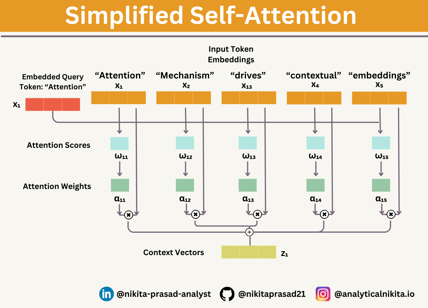
The input is a text (for example, a sentence like "Attention Mechanism drives contextual embedding") that has already been converted into token embeddings.
For instance, x1 is a d-dimensional vector representing the word "Attention", x2 for “Mechanism”, and so forth.
Goal: To compute context vectors, zi for each input sequence element xi in x1 to xT, where z and x have the same dimension.
The code below walks through the figure above step by step:
In the case of the tensor shown above, each row represents a word, and each column represents an embedding dimension:
We use input sequence element 1, x1, as an example to compute context vector z1; later, we will generalize this to compute all context vectors.
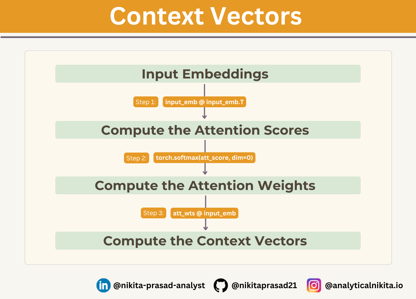
Step 1: Attention Scores (ω)
The first step is to compute the unnormalized attention scores by computing the dot product between the query x1 and all other input tokens:
Raw, unnormalized values that indicates how relevant one input element is to another.
Computed by comparing the query vector (Q) of one element with the key vector (K) of all element.
query = input_emb[0]  # 1st input token is the query

attn_scores_1 = torch.empty(input_emb.shape[0])
for i, x_i in enumerate(input_emb):
    attn_scores_1[i] = torch.dot(x_i, query) # dot product (transpose not necessary here since they are 1-dim vectors)

print(attn_scores_1)

# Output: tensor([0.6658, 0.8154, 0.8938, 0.7887, 0.3466])
Note: A dot product is used for multiplying two vectors elements-wise and summing the resulting products.
Step 2: Attention Weights (α)
It represent the relative importance of one element to another in a probabilistic manner (value between 0 to 1).
Note: Larger weights means greater relevance.
Let’s normalize the unnormalized attention scores ("omegas", ω) so that they sum up to 1:
Note: It is recommended, to use the softmax function for normalization, which is better at handling extreme values and has more desirable gradient properties during training.
So, let’s use the PyTorch implementation of softmax for scaling, which also normalizes the vector elements such that they sum up to 1:
The input embedding vectors are converted to the context vector.
It aims to capture both semantic and syntactic information from the input embeddings.
It is the key component that encodes the weighted representation of the input sequence, to capture most relevant information for each element in the sequence by considering its relationship with all other tokens.
Note: Context size is the maximum number of previous tokens the LLM looks at before predicting next token.
Let’s, compute the context vector z1 by multiplying the embedded input tokens, xi with the attention weights and sum the resulting vectors:
query = input_emb[0] # 1st input token is the query

context_vec_1 = torch.zeros(query.shape)
for i,x_i in enumerate(input_emb):
    context_vec_1 += attn_weights_1[i]*x_i

print(context_vec_1)

# Output: tensor([0.3897, 0.5495, 0.6587])
The model now has a weighted understanding of the input sequence.
Computing Attention Weights for All Input Tokens
Above, we computed the attention weights and context vector for input 1.
Next, let’s generalizing this computation for all tokens in the input embeddings.
Applying step 1 to all pairwise elements to compute the unnormalized attention score matrix: